Intro
This post describes peptide docking using Autodock CrankPep (ADCP) (Version 1.0 rc1), some post-processing including converting the output structure of the docked peptide into a charged RDKit molecule, and finally a very primitive “induced-fit” refinement using the local optimization function, optimize, from AutoDock Vina’s Python bindings. The efforts were based on the current major version of ADCP as of Oct 2023 with the intent to enable post-processing of ADCP outcomes by Vina and RDKit in Python.
The provided example is based on an experimental structure of Spt6-Iws1(Spn1) complex from E. cuniculi (PDB ID: 2XPP). The crystal structure 2XPP contains two chains: The longer one is Iws1 and will be the receptor in the docking calculation. The shorter one is a truncated form of Spt6. In addition to the mentioned structure, the Spt6-Iws1 complex is also observed in a high-res EM structure of actively working RNA polymerase II elongation complex (PDB ID: 7XN7). The peptide sequence FFEIF is part of the IWS1-interacting domain of Spt6 in E. cuniculi. Similar sequences are present in Spt6 across different species, with a highly conserved F residue that fits the binding site on the Iws1 receptor. The presence of multiple F residues makes the 5-mer sequence from E. cuniculi an interesting sequence to explore in peptide docking calculations.
Overview
This post will walk you through a peptide docking project consisting of (1) docking calculation with ADCP, (2) post-processing with reduce, and (3) structure refinement and rescoring with Vina.
To reproduce the presented work, you must have the software dependencies:
- ADFR Suite (v1.0 rc1, including
ADCP,reduce,prepare_ligand,prepare_receptor) - Meeko (Python Bindings, v0.5)
- AutoDock Vina (Python Bindings, v1.2.5)
Associated Files
Contains input PDB files, 2xpp_iws1.pdb and 2xpp_FFEIF.pdb, for the peptide docking examples.
peptide-docking/
├── 2xpp_FFEIF.pdb
└── 2xpp_iws1.pdb
Table of Contents
- Step 1: Docking Calculation with ADCP
- Step 2: Post-processing with reduce
- Step 3: Local Optimization with Vina
Step 1: Docking Calculation with ADCP
In this step, we will perform docking calculations for a peptide from sequence FFEIF and the receptor Iws1 from crystal structure 2XPP. A top-ranked binding mode will be chosen for post-processing and optimization in the further steps.
Structure and Target Preparation
Following the steps in the ADCP documentation, we will generate the PDBQT files for the peptide and the receptor, and the TRG file for the receptor -
reduce 2xpp_iws1.pdb > 2xpp_recH.pdb;
It should be noted that reduce will not protonate any of the imidazole nitrogens on HIS sidechains, unless with option -NOFLIP (or -HIS or -BUILD).
reduce 2xpp_FFEIF.pdb > 2xpp_pepH.pdb;
prepare_receptor -r 2xpp_recH.pdb -o 2xpp_recH.pdbqt;
prepare_ligand -l 2xpp_pepH.pdb -o 2xpp_pepH.pdbqt;
agfr -r 2xpp_recH.pdbqt -l 2xpp_pepH.pdbqt -asv 1.1 -o 2xpp;
In addition to running with Shell (preferably zsh) scripts, such commands can always be executed from Jupyter Notebook -
import subprocess
from subprocess import PIPE
def shell(cmd):
    process = subprocess.Popen(cmd, shell=True, stdout = subprocess.PIPE, stderr = subprocess.PIPE)
    out, err = process.communicate()
    outlines = out.decode("utf-8").split("\n")
    errlines = err.decode("utf-8").split("\n")
    for line in outlines+errlines:
        print(line)
Docking Calculations
Running the docking calculations with insufficient scope (number of independent GA runs, as specified by -N) and depth (number of max. MC steps, as specified by -n) will result in less reproducible outcomes. Here is my recipe for the presented system, which I think will produce relatively reproducible results for 5-mer to 7-mer peptides -
#!/bin/zsh
adcp -t 2xpp.trg -s FFEIF -N 400 -n 20000000 -o dock1 -ref 2xpp_pepH.pdb -c 40 &> dock1.log;

adcp -t 2xpp.trg -s FFEIF -N 400 -n 20000000 -o dock2 -ref dock1_ranked_1.pdb -c 40 &> dock2.log;

dock1_rank="$(grep -m1 "| ref. |" dock1.log -a3 | tail -n1)";
S1="$(echo "${dock1_rank}" | awk '{split($0,a," "); print a[2]}')";
s1=$((S1));
dock2_rank="$(grep -m1 "| ref. |" dock2.log -a3 | tail -n1)";
S2="$(echo "${dock2_rank}" | awk '{split($0,b," "); print b[2]}')";
s2=$((S2));

cp dock2_ranked_1.pdb nc_ref.pdb;
if (( $s1 < $s2 )); then
  cp dock1_ranked_1.pdb nc_ref.pdb;
  else
fi

adcp -t 2xpp.trg -s FFEIF -N 400 -n 20000000 -o dock3 -ref nc_ref.pdb -nc 0.8 -c 40 &> dock3.log;
Method explained
- The population of initial conformer is set to be all-helical, as specified by the sequence in ALL-CAPS. Three docking calculations were performed in serial, each containing 400 independent GA runs with max. 20,000,000 MC steps per GA run.
- Docking Calculation #1 may use an arbitrarily placed (preferably folded in the desired way, if helical, coil or a specific secondary structure is expected) conformer of the peptide. The default RMSD clustering will be used after completion of all searches.
- Docking Calculation #2 uses the top-ranked conformer from Docking Calculation #2 and the default RMSD clustering.
- Docking Calculation #3 uses the conformer from Docking Calculations #1 and #2 that has the lowest printed affinity. The default contact-based clustering is used, assuming the selected conformer from the previous docking calculations has the native contacts. Outcomes from Docking Calculation #3 will be considered for post-processing and further optimization.
I perform the docking calculations in three replicates, but with different reference structures for clustering, because I think choice of reference might affect clustering and ranking, and often times there is no prior knowledge what the best conformation (folding) would be like for the sequences of interest (unless the calculation is strictly a re-docking, while this example is not), and no reference structure to start with for the native contact analysis. However, if the top-ranked binding modes can be found in three replicates and are ranked invariantly with choice of reference structure, then I would take them as reproducible top-ranked binding modes.
Below are the standard outputs I got for the top 10 binding modes from the example docking calculations -
dock1.log
mode |  affinity  | clust. | ref. | clust. | rmsd | best | energy | best |
     | (kcal/mol) | rmsd   | rmsd |  size  | avg. | rmsd |  avg.  | run  |
-----+------------+--------+------+--------+------+------+--------+------+
   1        -15.3     0.0     5.3    4873     5.3   3.7   -13.1    9724
   2        -15.0     4.7     2.6     113     2.7   1.8   -13.3    18101
   3        -15.0     3.5     3.9    3132     3.7   2.2   -12.8    19274
   4        -14.9     5.9     3.7    1753     3.7   2.5   -13.2    17920
   5        -14.8     6.4     5.3     385     5.2   4.7   -12.8    19910
   6        -14.8     6.4     5.0    1333     4.9   4.2   -12.6    35129
   7        -14.6     6.9     4.1    1023     4.0   2.6   -12.5    36704
   8        -14.6     4.1     3.4     554     3.4   1.6   -11.4    32717
   9        -14.4     5.9     2.2     748     2.5   1.5   -11.7    66771
  10        -14.2     5.2     4.9    1237     4.9   4.0   -12.3    55850
From the above outputs, we should see that compared to how it positioned in the crystal structure 2XPP, the peptide FFEIF adopts a different conformation or binding mode in the top-ranked pose with RMSD = 5.3 to the reference structure which is essentially from the crystal structure.
dock2.log
mode |  affinity  | clust. | ref. | clust. | rmsd | best | energy | best |
     | (kcal/mol) | rmsd   | rmsd |  size  | avg. | rmsd |  avg.  | run  |
-----+------------+--------+------+--------+------+------+--------+------+
   1        -15.3     0.0     0.1    4757     0.9   0.1   -13.2    17300
   2        -15.1     4.9     4.9     215     5.3   4.4   -12.7    66267
   3        -14.9     6.1     6.1    1464     6.1   5.3   -13.0    1767
   4        -14.8     4.0     3.9    3054     3.5   2.7   -12.9    24942
   5        -14.7     6.3     6.3    1549     6.5   6.0   -12.8    46071
   6        -14.5     6.5     6.5     539     6.5   5.6   -12.4    64089
   7        -14.3     6.9     6.9     869     6.9   6.0   -12.6    45899
   8        -14.2     6.8     6.8      40     6.9   6.4   -13.0    21812
   9        -14.2     5.1     5.1    1107     5.4   5.1   -12.3    65626
  10        -14.1     4.1     4.1     603     4.3   3.0   -11.4    63408
From the above outputs, we should see that the top-ranked pose in Docking Calculation #2 is highly consistent with the top-ranked pose in Docking Calculation #1, which is the reference structure here, with RMSD = 0.1.
dock3.log
mode |  affinity  | ref. | clust. | rmsd | energy | best |
     | (kcal/mol) | fnc  |  size  | stdv |  stdv  | run  |
-----+------------+------+--------+------+--------+------+
   1        -15.7    1.000    4190      NA      NA    33189
   2        -14.9    0.900    2183      NA      NA    41742
   3        -14.9    0.550    1546      NA      NA    42954
   4        -14.8    0.500    1238      NA      NA    66033
   5        -14.6    0.650      68      NA      NA    60254
   6        -14.5    0.550      43      NA      NA    53970
   7        -14.5    0.450      29      NA      NA    35465
   8        -14.4    0.600     618      NA      NA    51413
   9        -14.3    0.400     121      NA      NA    42604
  10        -14.3    0.550     138      NA      NA    16287
From the above outputs, we should see that the top-ranked pose in Docking Calculation #3 is still consistent with the top-ranked pose in Docking Calculations #1 and #2, for having the same (fraction = 1.000) native contacts.
Step 2: Post-processing with reduce
In this step, we will work on the top-ranked binding mode obtained from Docking Calculation #3, which was written to dock3_ranked_1.pdbqt. Because ADCP does not make indications on the tautomeric or protonation form of HIS (whether it is HIE/HID or HIP), the evaluation will be made in reduce on the combined structure of protein-peptide complex. The protonated complex will be the initial structure for local optimization in the next step.
Generate Combined Structure of the Protein-Peptide Complex
To begin with, we will make a combined structure of the protein-peptide complex, using the unprotonated protein structure 2xpp_iws1.pdb and the top-ranked peptide binding mode dock3_ranked_1.pdb. This can be done with a molecule editing tool, a text editing tool or by the following Python codes -
def order_pdb(input_pdb):
    resnum_list = []
    resblock_dict = {}
    with open(input_pdb,"r") as f:
        line = f.readline()
        while line:
            if line[:6] in ["ATOM  "]:
                resnum = line[22:26]
                if resnum not in resnum_list:
                    resnum_list.append(resnum)
                    resblock_dict[resnum] = [line] # residues must have unique residue numbers
                else:
                    resblock_dict[resnum].append(line)
            line = f.readline()
    ordered_pdb_block = []
    for resnum in resnum_list:
        ordered_pdb_block += resblock_dict[resnum]
    return ordered_pdb_block

def make_complex(receptor_pdb, ligand_pdb):
    # initialisation
    data = []

    # read receptor pdb
    with open(receptor_pdb,"r") as f:
        line = f.readline()
        while line:
            if line[:6]=="ATOM  ":
                data.append(line)
            line = f.readline()
    data.append("TER\n")

    # reorder atoms in ADCP output, add ligand pdb
    data += order_pdb(ligand_pdb)
    return data

with open("complex_1.pdb","w") as fw:
    for line in make_complex('2xpp_iws1.pdb', 'dock3_ranked_1.pdb'):
        fw.write(line)
    fw.write("TER\nEND\n")
In the above Python codes, the atoms in ADCP output file dock3_ranked_1.pdb are re-ordered by residue as required by reduce.
Protonate the Protein-Peptide Complex
Next, we will run reduce on the complex structure complex_1.pdb. We will use -NOFLIP option to build hydrogens for HIS sidechain nitrogens -
reduce -NOFLIP complex_1.pdb > complex_1H.pdb
Write the Updated Receptor and Peptide Ligand PDBQT File
Finally, we will split the protonated protein-peptide complex complex_1H.pdb into protein and peptide ligand. We will also correct the residue names for HIS residues according to their tautomeric and protonation forms. The following Python code will generate the protein PDB file complex_1H_rec.pdb and receptor PDB file complex_1H_pep.pdb with corrected residue names -
# assigns HIE/HID/HIP in protonated protein or peptide pdb files
def assign_his(input_pdb_block):
    resnum_list = []
    resblock_dict = {}
    resname_dict = {}
    for line in input_pdb_block:
        if line[:6] in ["ATOM  "]:
            resnum = line[22:26]
            if resnum not in resnum_list:
                resnum_list.append(resnum)
                resblock_dict[resnum] = [line] # residues must have unique residue numbers
                resname_dict[resnum] = line[17:20] # residue names must present in res_smi
            else:
                resblock_dict[resnum].append(line)
    new_pdb_block = []
    for resnum in resnum_list:
        newname = "HID" # assumes HID
        if resname_dict[resnum] in ["HIS"]:
            resblock = resblock_dict[resnum]
            anames = [aline[12:16] for aline in resblock]
            if " HE2" in anames:
                if " HD1" not in anames:
                    newname = "HIE"
                else:
                    newname = "HIP"
            resblock_dict[resnum] = [aline.replace("HIS",newname) for aline in resblock]
        new_pdb_block += resblock_dict[resnum]
    return new_pdb_block

## assumes receptor appears before peptide
## assumes TER presents at the end of receptor
rec, pep = [[],[]]
with open("complex_1H.pdb","r") as f:
    line = f.readline()
    while line:
        if line[:6]=="ATOM  ":
            rec.append(line)
        else:
            if line[:3]=="TER":
                break
        line = f.readline()
    while line:
        if line[:6]=="ATOM  ":
            pep.append(line)
        line = f.readline()

with open("complex_1H_rec.pdb","w") as fw:
    for line in assign_his(rec):
        fw.write(line)
# write pep
with open("complex_1H_pep.pdb","w") as fw:
    for line in assign_his(pep):
        fw.write(line)
Now, we may redo receptor preparation with prepare_receptor -
prepare_receptor -r complex_1H_rec.pdb -o complex_1H_rec.pdbqt
In theory, mk_prepare_receptor.py could do the same thing -
mk_prepare_receptor.py \
--pdb complex_1H_rec.pdb -o complex_1H_rec \
--box_size 30 30 30 --box_center 20.076 10.981 27.791 --skip_gpf
mk_prepare_receptor.py does not tolerate missing and/or incomplete capping groups, so it won’t work for complex_1H_rec.pdb.
The peptide ligand preparation can be done from a PDB file, using prepare_peptide_ligand.py I propose to prepare the peptide ligand PDBQT file from a PDB file -
from prepare_peptide_ligand import *
with open("complex_1H_pep.pdbqt","w") as fw:
    fw.write(mode_to_pdbqt_string("complex_1H_pep.pdb"))
Step 3: Local Optimization with Vina
In this step, we will use the protein receptor PDBQT file complex_1H_rec.pdbqt and the peptide ligand PDBQT file complex_1H_pep.pdbqt from the previous step and use Vina to perform local optimization.
Rigid Receptor Local Optimization
Below is the Python code to perform the local minimization based on the Vina Documentation on Python Scripting -
from vina import Vina

v = Vina(sf_name='vina')

v.set_receptor('complex_1H_rec.pdbqt')

v.set_ligand_from_file('complex_1H_pep.pdbqt')
v.compute_vina_maps(center=[20.076, 10.981, 27.791], box_size=[30, 30, 30])

# Score the current pose
energy = v.score()
print('Score before minimization: ', energy)

# Minimized locally the current pose
energy_minimized = v.optimize()
print('Score after minimization : ', energy_minimized)
v.write_pose('mode_1_minimized.pdbqt', overwrite=True)
Outputs
Score before minimization:  [-4.133 -9.087  0.     0.     0.    14.634  4.954 14.634]
Score after minimization :  [ -5.778 -12.703   0.      0.      0.     -2.916   6.925  -2.916]
Computing Vina grid ... done.
Performing local search ... done.
From the above outputs, we should see that Vina’s optimize function has improved lig_inter energy from -9.087 to -12.703, indicating increased protein-peptide interactions after optimization. The lig_intra energy has also been improved from 14.634 to -2.916, suggesting more stable conformation of the peptide ligand.
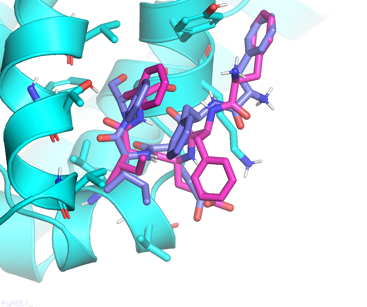
Below is an overlay picture of the top-ranked pose, before (cyan) vs. after (magenta) the local optimization:
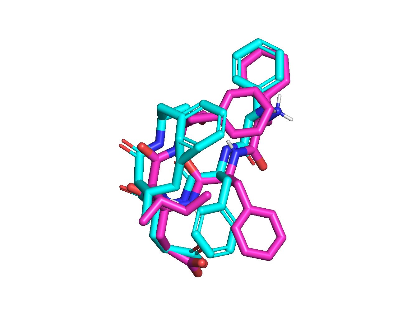
It can be seen from the overlay that, the major improvement is the spacing of atoms in peptide residues I and F that were too close in the original ADCP output.
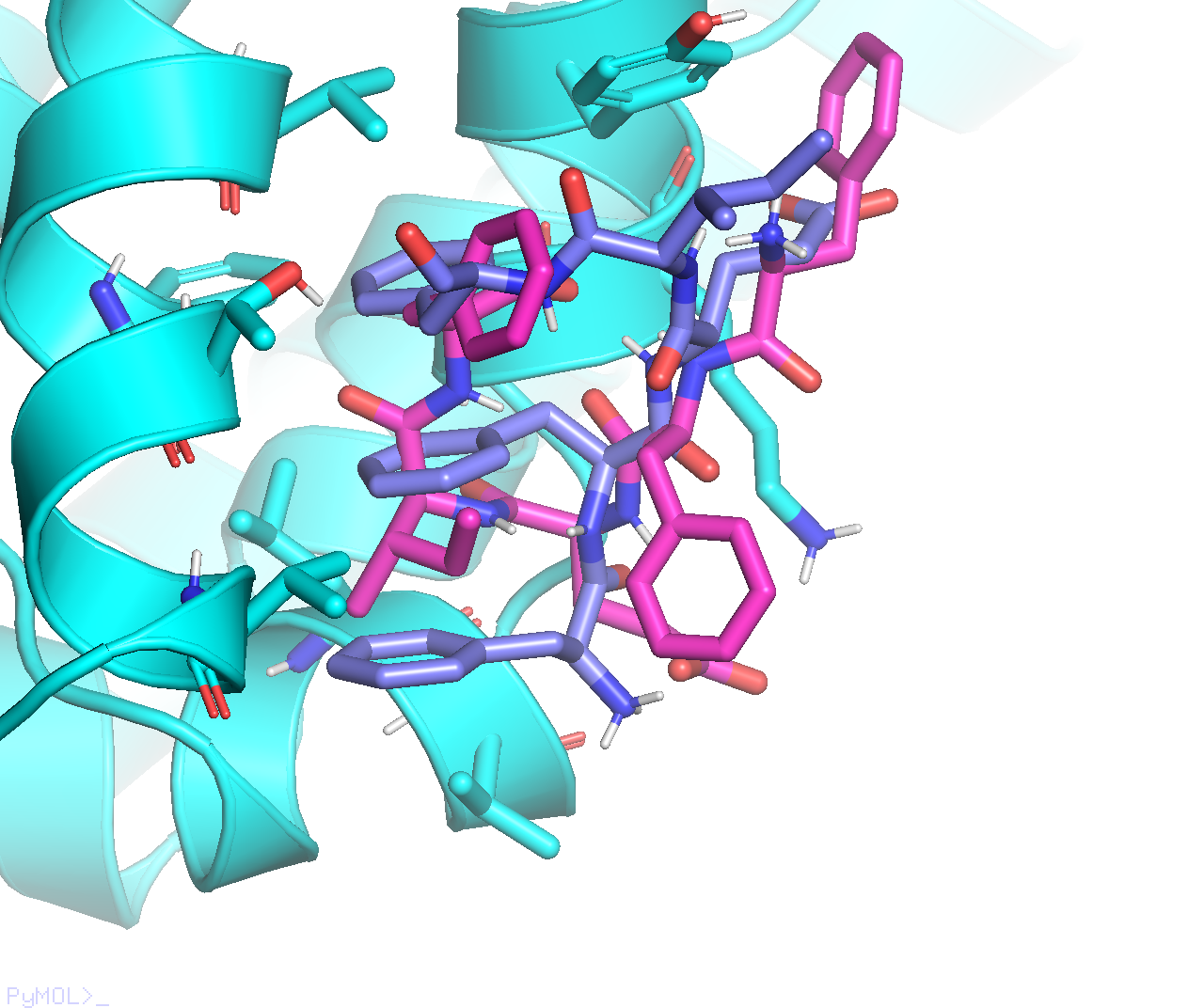
And an overlay picture of the minimized top-ranked pose (magenta) and the position of sequence FFEIF in the crystal structure (green):
It can be seen from the overlay that, residue I is docked at almost the native position. The last (5th) residue F is docked at a near native position, but in a different orientation, probably due to the absence of the subsequent residues. Residue E is docked to interact with a positively charged residue K in the protein receptor. In crystal structure 2XPP, the native orientation of E does not have an apparent interaction with a receptor residue.
Compare with Docking in Vina
With the protein receptor PDBQT file complex_1H_rec.pdbqt and the peptide ligand PDBQT file complex_1H_pep.pdbqt, it is also possible to perform docking with Vina in Python -
from vina import Vina

v = Vina(sf_name='vina')

v.set_receptor('complex_1H_rec.pdbqt')

v.set_ligand_from_file('complex_1H_pep.pdbqt')
v.compute_vina_maps(center=[20.076, 10.981, 27.791], box_size=[30, 30, 30])

v.dock(exhaustiveness=32, n_poses=20)
v.write_poses('2xpp_ligand_vina_out.pdbqt', n_poses=5, overwrite=True)
Outputs
mode |   affinity | dist from best mode
     | (kcal/mol) | rmsd l.b.| rmsd u.b.
-----+------------+----------+----------
   1       -6.518          0          0
   2       -6.414      2.764      8.073
   3       -6.405      2.881      7.948
   4       -6.354       2.37      5.629
   5       -6.352      3.707      9.795
   6       -6.278      2.483      8.303
   7       -6.267      2.609      7.185
   8       -6.258      3.226      9.151
   9       -6.255      2.494      4.451
  10        -6.19      2.497      9.221
  11       -6.136      2.464      5.836
  12       -6.107      2.744      6.391
  13       -6.077      2.758      6.186
  14       -6.067      2.589      4.446
  15       -6.058      2.308      8.259
  16       -6.038      2.367      8.083
  17       -6.035      2.718      6.809
  18       -6.032      2.075      3.957
  19       -6.008      2.683      5.735
  20       -5.976      3.327      8.089
Performing docking (random seed: -1838194651) ...
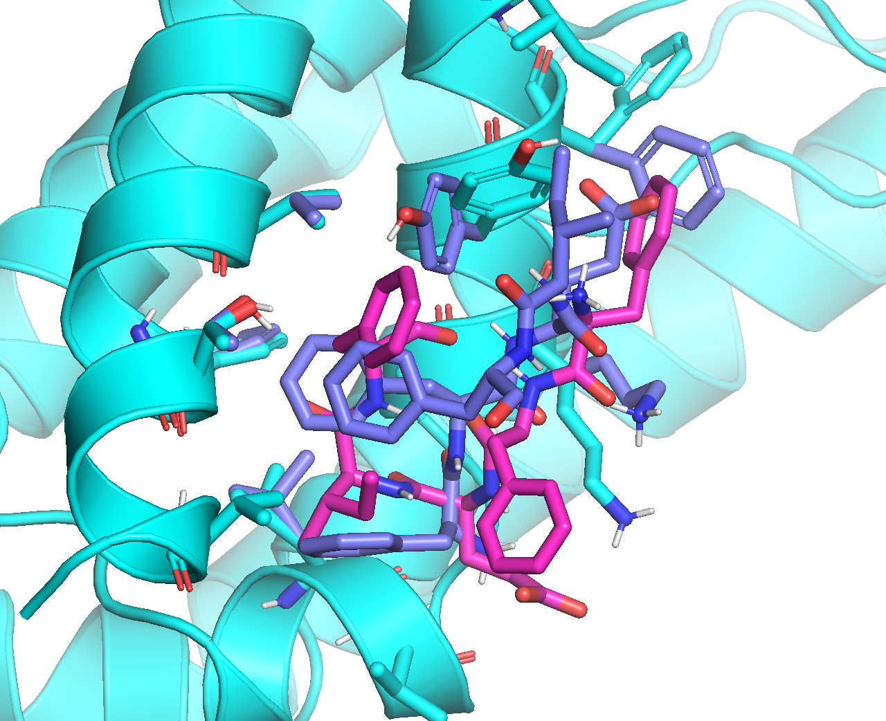
From the above docking calculation, I found that Vina’s output mode#2 (purple) is similar to ADCP’s top-ranked mode (magenta) we have been working on:
While Vina’s output mode#1 (purple) adopts a very interesting conformation, with three F residues stacked on top of each other:
Flexible Receptor Local Optimization
In the final section of this post, we will show a primitive “induced-fit” optimization by performing local optimization with flexible receptor sidechains, using Vina’s optimize in Python. To begin with, we will run receptor preparation with mk_prepare_receptor.py for complex_1H_rec.pdbqt and a few selected sidechains based on distances and interactions with the peptide ligand in the binding mode showed in complex_1H_pep.pdbqt.
First, for the receptor preparation -
mk_prepare_receptor.py \
--pdbqt complex_1H_rec.pdbqt -o complex_1H_mk \
-f A:TYR:164 -f A:LYS:161 -f A:THR:188 \
-f A:PHE:165 -f A:LEU:154 -f A:VAL:184 \
-f A:TRP:187 \
--box_size 30 30 30 --box_center 20.076 10.981 27.791 --skip_gpf
Next, we will perform local optimization in Python -
v = Vina(sf_name='vina')

v.set_receptor(rigid_pdbqt_filename='complex_1H_mk_rigid.pdbqt', flex_pdbqt_filename='complex_1H_mk_flex.pdbqt')

v.set_ligand_from_file('complex_1H_pep.pdbqt')
v.compute_vina_maps(center=[20.076, 10.981, 27.791], box_size=[30, 30, 30])

# Score the current pose
energy = v.score()
print('Score before minimization: ', energy)

# Minimized locally the current pose
energy_minimized = v.optimize()
print('Score after minimization : ', energy_minimized)
v.write_pose('mode_1_flex_minimized.pdbqt', overwrite=True)
Outputs
Computing Vina grid ... Score before minimization:  [-4.03  -6.87  -1.391 -7.68  -1.668 14.634  4.829  5.883]
Score after minimization :  [ -5.766  -7.104  -5.029  -8.532  -1.876  -3.627   6.911 -13.491]
done.
Performing local search ... done.
And finally, we can run a docking calculation immediately after the local optimization -
v.dock(exhaustiveness=32, n_poses=20)
v.write_poses('2xpp_ligand_vina_flex_out.pdbqt', n_poses=5, overwrite=True)
Outputs
mode |   affinity | dist from best mode
     | (kcal/mol) | rmsd l.b.| rmsd u.b.
-----+------------+----------+----------
   1        -6.95          0          0
   2       -6.776      1.798      6.518
   3       -6.694      1.918       3.56
   4       -6.653      2.024       6.89
   5       -6.599      2.286      4.095
   6       -6.558      1.804      4.914
   7       -6.485       1.97      5.734
   8       -6.479      2.073      5.386
   9       -6.477      1.737      3.347
  10       -6.449      2.158       4.21
  11       -6.429      1.692      3.516
  12       -6.426      1.308      2.006
  13       -6.403      2.009      4.388
  14       -6.262      2.244      6.838
  15       -6.213      2.536      6.052
  16       -6.205      2.515       6.28
  17       -6.201      2.068       5.04
  18       -6.189      1.863      4.501
  19       -6.125      2.254      3.969
  20       -6.077      2.129      6.394
Performing docking (random seed: 196250666) ...
To summarize, visual comparisons are provided for the following generated structures:
- Minimized ADCP top binding mode with rigid receptor (magenta).
- Minimized ADCP top binding mode with flexible receptor (yellow).
- Top binding modes from Vina’s docking with flexible receptor (purple).
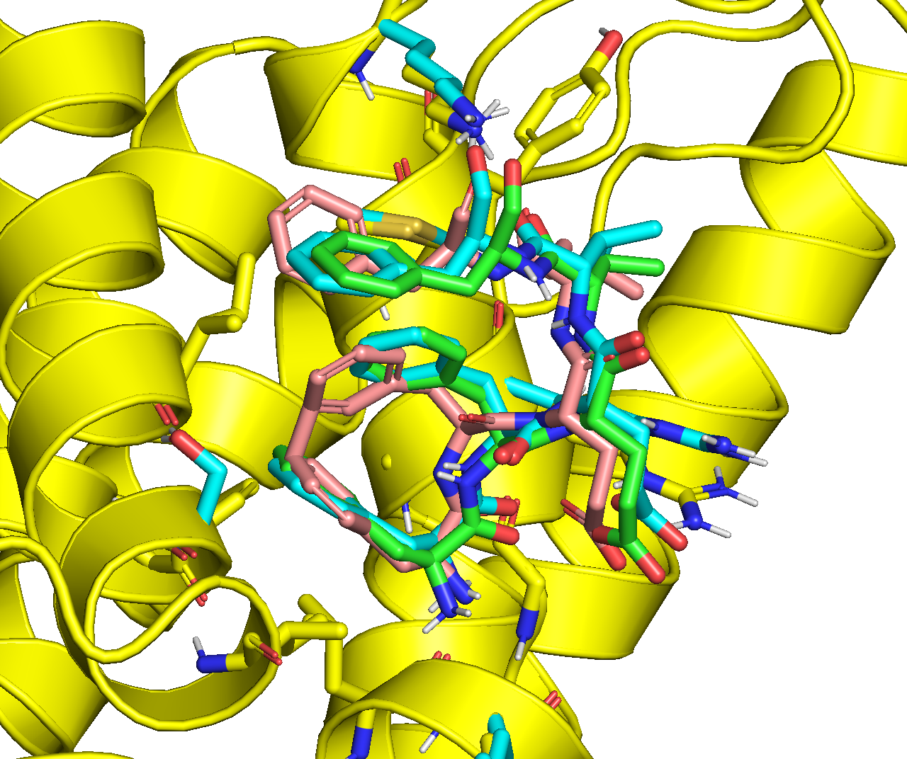
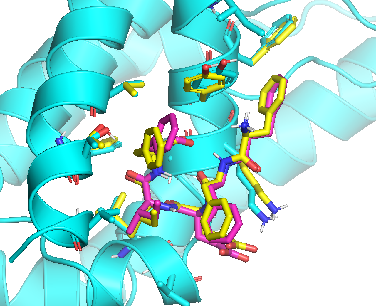
Below is an overlay of the ADCP top binding modes that were minimized with rigid receptor (magenta) and flexible receptor (yellow):
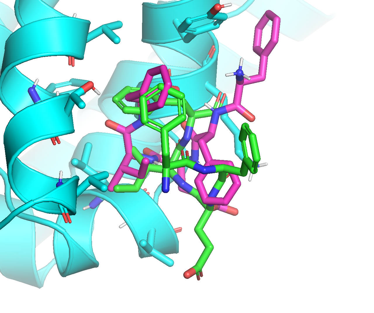
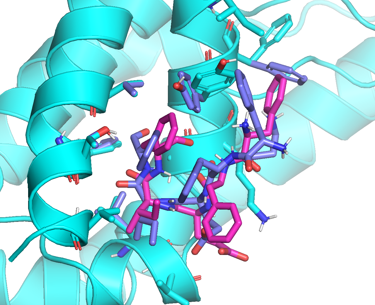
Below is an overlay of the minimized ADCP top binding mode with rigid receptor (magenta), and Vina’s #2 binding mode with flexible receptor (purple). Although some of the receptor sidechains are positioned differently, the binding modes of the peptide ligand are generally consistent with each other:
Below is an overlay of the minimized ADCP top binding mode with rigid receptor (magenta), and Vina’s #1 binding mode with flexible receptor (purple). Both the receptor sidechains and the binding modes of the peptide ligand are substantially different: